首页
— 线性规划模型及编程求解 —
Haifeng Xu
(hfxu@yzu.edu.cn)
This slide is based on the book:
赵静、但琦 主编《数学建模与数学实验》(第4版)
线性规划
线性规划
建立优化问题的数学模型, 首先要确定问题的决策变量, 决策变量含有多个因素, 因此一般用向量 $\vec{x}=(x_1,x_2,\ldots,x_n)^T$ 来表示. 当然这些 $x_i$ 是有限定范围的. 设 $\vec{x}\in\Omega$, 称 $\Omega$ 为可行域.
另外这些变量 $x_i$ 之间满足一些约束条件, 记为 $g_i(\vec{x})\leqslant 0$, $(i=1,2,\ldots,m)$. 从而数学模型可以表示如下:
\[
\begin{aligned}
&\min_{\vec{x}\in\Omega} z=f(\vec{x})\qquad(1)\\
\text{s. t.} \ &g_i(\vec{x})\leqslant 0,\quad\text{for}\ i=1,2,\ldots,m.\qquad(2)
\end{aligned}
\]
由上述 (1) 和 (2) 组成的模型属于约束优化, 若只有 (1) 式, 则称为无约束优化, $f(x)$ 称为目标函数, 而 $g_i(\vec{x})\leqslant 0$, $(i=1,2,\ldots,m)$ 称为约束条件.
决策变量、目标函数、约束条件构成了线性规划的三个基本要素.
建立线性规划的三个基本步骤
- Step1. 找出待定的未知变量(决策变量), 并用代数符号表示它们.
- Step2. 找出问题中所有的限制或约束, 写出未知变量的线性方程或线性不等式.
- step3. 找到模型的目标或判据, 写成决策变量的线性函数, 以便求出最大值或最小值.
例子1
例1
生产炊事用具需要两种资源————劳动力和原材料,某公司指定生产计划,生产三种不同产品,生产管理部门提供的数据如下:
| 每件产品所需 ... \ 产品类型 |
A |
B |
C |
| 劳动力(小时·件${}^{-1}$) |
7 |
3 |
6 |
| 原材料(千克·件${}^{-1}$) |
4 |
4 |
5 |
| 利润(元·件${}^{-1}$) |
4 |
2 |
3 |
每天供应原材料 200kg, 每天可供使用的劳动力为 150h. 建立线性规划模型, 使总收益最大, 并求各种产品的日产量.
Step 1. 确定决策变量
要求的未知变量是三个产品的日产量. 用代数符号 $x_A, x_B, x_C$ 分别表示 $A,B,C$ 三种产品的日产量.
Step 2. 确定约束条件.
在这个问题中, 约束条件可用劳动力和原材料来限制:
\[
\begin{aligned}
\text{劳动力:}\ 7x_A+3x_B+6x_C \leqslant 150,\\
\text{原材料:}\ 4x_A+4x_B+5x_C \leqslant 200,\\
\end{aligned}
\]
Step 3. 确定目标函数.
本问题的目标是使总收益最大, 总收益为
\[
Z=4x_A+2x_B+3x_C.
\]
得到线性规划模型
\[
\max Z=4x_A+2x_B+3x_C
\]
\[
\text{s.t.}\
\begin{cases}
4x_A+4x_B+5x_C \leqslant 200,\\
7x_A+3x_B+6x_C \leqslant 150,\\
x_A, x_B, x_C\geqslant 0.
\end{cases}
\]
实验(用MATLAB或Lingo解决)
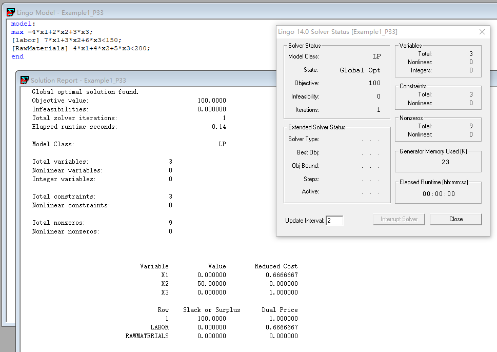
model:
max =4*x1+2*x2+3*x3;
[labor] 7*x1+3*x2+6*x3<150;
[RawMaterials] 4*x1+4*x2+5*x3<200;
end
运行 Lingo
运行结果
注意[]中不能有空格, 否则语法错误, 比如不能写成[Raw materials]
例子2
广告手段的选择
一家广告公司想在电视、广播、杂志上做广告,其目的是尽可能多地招揽顾客。下面是市场调查结果:
| |
电视 |
广播 |
杂志 |
| |
白天 |
最佳时间 |
| 一次广告费用(千元) |
40 |
75 |
30 |
15 |
| 受每次广告影响的顾客数(千人) |
400 |
900 |
500 |
200 |
| 受每次广告影响的女顾客数(千人) |
300 |
400 |
200 |
100 |
这家公司希望广告费用不超过 800(千元),还要求:
- 至少要有200万女性收看广告;
- 电视广告费用不超过 500(千元);
- 电视广告白天至少播出 3 次,最佳时间至少播出 2 次;
- 通过广播、杂志做的广告要重复 5 到 10 次。
建立模型
令 $x_1,x_2,x_3,x_4$ 分别表示白天电视、最佳时间电视、广播、杂志广告的次数。于是广告经费的约束条件为:
\[
40x_1+75x_2+30x_3+15x_4\leqslant 800.
\]
受广告影响的女顾客数的约束条件为:
\[
300x_1+400x_2+200x_3+100x_4\geqslant 2000.
\]
电视广告的约束条件为:
\[
\begin{aligned}
40x_1+75x_2&\leqslant 500,\\
x_1&\geqslant 3,\\
x_2&\geqslant 2.
\end{aligned}
\]
由于广播和杂志广告的次数都要在 5 到 10 之间, 于是
\[
\begin{aligned}
5\leqslant x_3\leqslant 10,\\
5\leqslant x_4\leqslant 10,
\end{aligned}
\]
潜在的顾客数: $Z=400x_1+900x_2+500x_3+200x_4$. 因此完整的线性规划如下:
\[
\max\ Z=400x_1+900x_2+500x_3+200x_4
\]
\[
\text{s.t.}\
\begin{cases}
40x_1+&75x_2 +&30x_3 +&15x_4 &\leqslant 800,\\
300x_1+&400x_2+&200x_3+&100x_4&\geqslant 2000,\\
40x_1 +&75x_2 & & &\leqslant 500,\\
x_1 & & & &\geqslant 3,\\
& x_2 & & &\geqslant 2,\\
& &x_3 & &\geqslant 5,\\
& &x_3 & &\leqslant 10,\\
& & &x_4 &\geqslant 5,\\
& & &x_4 &\leqslant 10,\\
& & & x_i&\geqslant 0,\ i=1,2,3,4.
\end{cases}
\]
实验
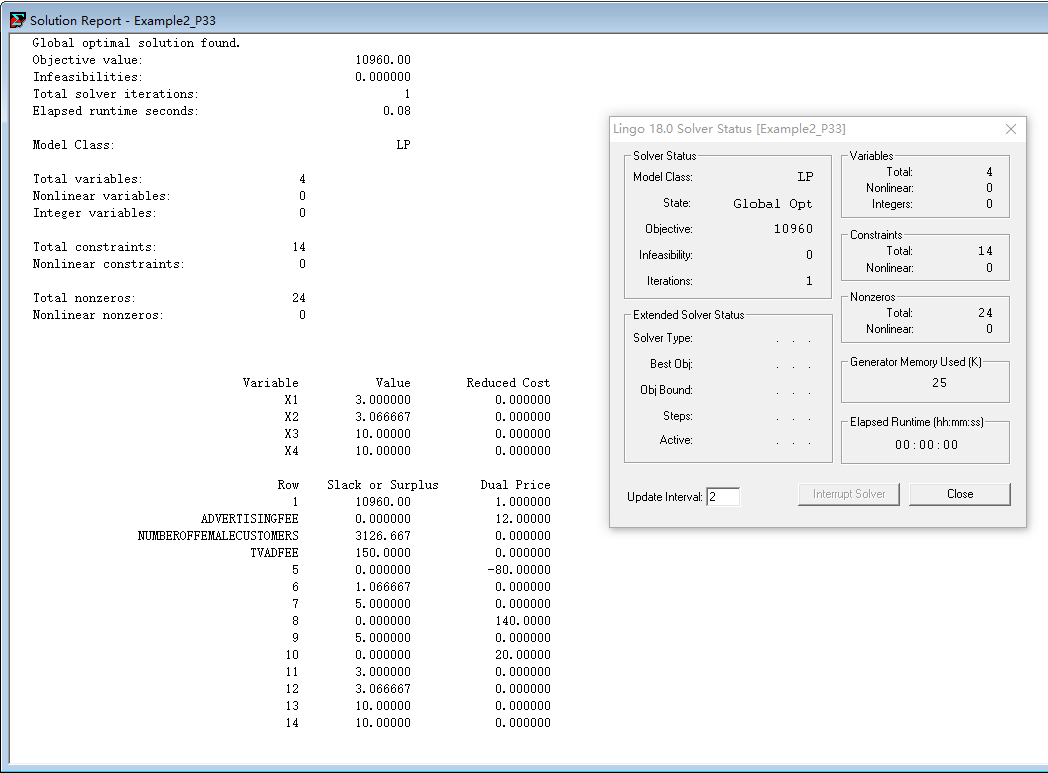
model:
max = 400*x1+900*x2+500*x3+200*x4;
[AdvertisingFee] 40*x1+75*x2+30*x3+15*x4<=800;
[NumberOfFemaleCustomers] 300*x1+400*x2+200*x3+100*x4>=2000;
[TVAdFee] 40*x1+75*x2<=500;
x1>=3;
x2>=2;
x3>=5;
x3<=10;
x4>=5;
x4<=10;
x1>=0;
x2>=0;
x3>=0;
x4>=0;
end
运行结果
任务分配问题
任务分配问题
某车间有甲、乙两台机床, 可用于加工三种工件. 假定
- 这两台车床的可用“台时数”分别为 800 和 900,
- 三种工件的数量分别为 400、600和500,
- 且已知用两种不同车床加工单位数量不同工件所需的台时数和加工费用如下表.
问怎样分配车床的加工任务, 才能既满足加工工件的要求, 又使加工费用最低.
| 车床类型 |
单位工件所需加工台时数 |
单位工件的加工费用 |
可用台时数 |
| |
工件1 |
工件2 |
工件3 |
工件1 |
工件2 |
工件3 |
|
| 甲 |
0.4 |
1.1 |
1.0 |
13 |
9 |
10 |
800 |
| 乙 |
0.5 |
1.2 |
1.3 |
11 |
12 |
8 |
900 |
建立模型
设在甲车床上加工工件1、2、3的数量分别为 $x_1$, $x_2$, $x_3$, 在乙车床上加工工件1、2、3的数量分别为 $x_4$, $x_5$, $x_6$. 可建立以下线性规划模型:
\[
\min z=13x_1+9x_2+10x_3+11x_4+12x_5+8x_6
\]
\[
\text{s.t.}\
\begin{cases}
x_1+x_4=400,\\
x_2+x_5=600,\\
x_3+x_6=500,\\
0.4x_1+1.1x_2+x_3\leqslant 800,\\
0.5x_4+1.2x_5+1.3x_6\leqslant 900,\\
x_i\geqslant 0,\ i=1,2,\ldots,6.
\end{cases}
\]
可改写为
\[
\min z=\begin{pmatrix}13& 9& 10& 11& 12& 8\end{pmatrix}
\begin{pmatrix}
x_1\\
x_2\\
x_3\\
x_4\\
x_5\\
x_6\\
\end{pmatrix}
\]
使满足下面的条件
\[
\begin{pmatrix}
0.4& 1.1& 1& 0& 0& 0\\
0& 0& 0& 0.5& 1.2& 1.3
\end{pmatrix}
\begin{pmatrix}
x_1\\
x_2\\
x_3\\
x_4\\
x_5\\
x_6\\
\end{pmatrix}
\leqslant
\begin{pmatrix}
800\\
900
\end{pmatrix}
\]
\[
\begin{pmatrix}
1\ \ 0\ \ 0\ \ 1\ \ 0\ \ 0\\
0\ \ 1\ \ 0\ \ 0\ \ 1\ \ 0\\
0\ \ 0\ \ 1\ \ 0\ \ 0\ \ 1\\
\end{pmatrix}
\begin{pmatrix}
x_1\\
x_2\\
x_3\\
x_4\\
x_5\\
x_6\\
\end{pmatrix}
=
\begin{pmatrix}
400\\
600\\
500\\
\end{pmatrix}
\]
使用 Matlab 解决
% sec3_2_exmp1.m
% Page 35
% 使用MATLAB优化工具箱求解线性规划问题.

f=[13 9 10 11 12 8];
A=[0.4 1.1 1 0 0 0;
    0 0 0 0.5 1.2 1.3];
b=[800; 900];
Aeq=[1 0 0 1 0 0;
     0 1 0 0 1 0;
     0 0 1 0 0 1];
beq=[400; 600; 500];
vlb=zeros(6,1);
vub=[];
[x,fval]=linprog(f,A,b,Aeq,beq,vlb,vub)
运行结果:
>> sec3_2_exmp1
警告: Your current settings will run a different algorithm ('dual-simplex') in a future release.

> In linprog (line 204)
  In sec3_2_exmp1 (line 15)
Optimization terminated.
x =
    0.0000
  600.0000
    0.0000
  400.0000
    0.0000
  500.0000
fval =
   1.3800e+04
>>
关于 linprog 的帮助
>> help linprog
 linprog Linear programming.
    X = linprog(f,A,b) attempts to solve the linear programming problem:

             min f'*x    subject to:   A*x <= b
              x

    X = linprog(f,A,b,Aeq,beq) solves the problem above while additionally
    satisfying the equality constraints Aeq*x = beq. (Set A=[] and B=[] if
    no inequalities exist.)

    X = linprog(f,A,b,Aeq,beq,LB,UB) defines a set of lower and upper
    bounds on the design variables, X, so that the solution is in
    the range LB <= X <= UB. Use empty matrices for LB and UB
    if no bounds exist. Set LB(i) = -Inf if X(i) is unbounded below;
    set UB(i) = Inf if X(i) is unbounded above.

    X = linprog(f,A,b,Aeq,beq,LB,UB,X0) sets the starting point to X0. This
    option is only available with the active-set algorithm. The default
    interior point algorithm will ignore any non-empty starting point.

    X = linprog(PROBLEM) finds the minimum for PROBLEM. PROBLEM is a
    structure with the vector 'f' in PROBLEM.f, the linear inequality
    constraints in PROBLEM.Aineq and PROBLEM.bineq, the linear equality
    constraints in PROBLEM.Aeq and PROBLEM.beq, the lower bounds in
    PROBLEM.lb, the upper bounds in  PROBLEM.ub, the start point
    in PROBLEM.x0, the options structure in PROBLEM.options, and solver
    name 'linprog' in PROBLEM.solver. Use this syntax to solve at the
    command line a problem exported from OPTIMTOOL.

    [X,FVAL] = linprog(f,A,b) returns the value of the objective function
    at X: FVAL = f'*X.

    [X,FVAL,EXITFLAG] = linprog(f,A,b) returns an EXITFLAG that describes
    the exit condition. Possible values of EXITFLAG and the corresponding
    exit conditions are

      1  linprog converged to a solution X.
      0  Maximum number of iterations reached.
     -2  No feasible point found.
     -3  Problem is unbounded.
     -4  NaN value encountered during execution of algorithm.
     -5  Both primal and dual problems are infeasible.
     -7  Magnitude of search direction became too small; no further
          progress can be made. The problem is ill-posed or badly
          conditioned.

    [X,FVAL,EXITFLAG,OUTPUT] = linprog(f,A,b) returns a structure OUTPUT
    with the number of iterations taken in OUTPUT.iterations, maximum of
    constraint violations in OUTPUT.constrviolation, the type of
    algorithm used in OUTPUT.algorithm, the number of conjugate gradient
    iterations in OUTPUT.cgiterations (= 0, included for backward
    compatibility), and the exit message in OUTPUT.message.

    [X,FVAL,EXITFLAG,OUTPUT,LAMBDA] = linprog(f,A,b) returns the set of
    Lagrangian multipliers LAMBDA, at the solution: LAMBDA.ineqlin for the
    linear inequalities A, LAMBDA.eqlin for the linear equalities Aeq,
    LAMBDA.lower for LB, and LAMBDA.upper for UB.

    NOTE: the interior-point (the default) algorithm of linprog uses a
          primal-dual method. Both the primal problem and the dual problem
          must be feasible for convergence. Infeasibility messages of
          either the primal or dual, or both, are given as appropriate. The
          primal problem in standard form is
               min f'*x such that A*x = b, x >= 0.
          The dual problem is
               max b'*y such that A'*y + s = f, s >= 0.

    See also quadprog.

    linprog 的参考页
例2
例2
某厂每日 8 小时的产量不低于 1800 件. 为了进行质量控制, 计划聘请两种不同水平的检验员. 且每种检验员的日产量不高于 1800 件.
- 一级检验员的标准为: 速度25件/小时, 正确率 98%, 计时工资4元/小时;
- 二级检验员的标准为: 速度15件/小时, 正确率 95%, 计时工资3元/小时;
- 检验员每错检一次, 工厂要损失 2 元.
为使总检验费用最省, 该工厂应聘请一级、二级检验员各几名?
解
设需要一级和二级检验员的人数分别为 $x_1$, $x_2$, 则应付检验员的工资为
\[
8\times 4\times x_1+8\times 3\times x_2=32x_1+24x_2.
\]
因检验员错检而造成的损失为
\[
(8\times 25\times 2\%\times x_1+8\times 15\times 5\%\times x_2)\times 2=8x_1+12x_2.
\]
故目标函数为
\[
\min z=(32x_1+24x_2)+(8x_1+12x_2)=40x_1+36x_2.
\]
约束条件为
\[
\begin{cases}
8\times 25\times x_1+8\times 15\times x_2\geqslant 1800,\\
8\times 25\times x_1\leqslant 1800,\\
8\times 15\times x_2\leqslant 1800,\\
x_i\geqslant 0,\quad i=1,2.
\end{cases}
\]
即得线性规划模型
\[
\min z=40x_1+36x_2
\]
\[
\text{s.t.}
\begin{cases}
5x_1+3x_2\geqslant 45,\\
x_1\leqslant 9,\\
x_2\leqslant 15,\\
x_i\geqslant 0,\quad i=1,2.
\end{cases}
\]
改写成
\[
\min z=\begin{pmatrix}
40 & 36
\end{pmatrix}
\begin{pmatrix}
x_1\\
x_2\\
\end{pmatrix}
\]
\[
\text{s.t.}
\begin{cases}
\begin{pmatrix}
-5 & -3
\end{pmatrix}
\begin{pmatrix}
x_1\\
x_2\\
\end{pmatrix}\leqslant -45\\
\begin{pmatrix}
0\\
0\\
\end{pmatrix}
\leqslant
\begin{pmatrix}
x_1\\
x_2\\
\end{pmatrix}
\leqslant
\begin{pmatrix}
9\\
15\\
\end{pmatrix}
\end{cases}
\]
使用 Matlab 解决, 编写 M 文件.
% P.37
%
c=[40 36];
A=[-5 -3];
b=[-45];
Aeq=[];
beq=[];
vlb=zeros(2,1);
vub=[9;15];
%然后调用linprog函数
[x,fval]=linprog(c,A,b,Aeq,beq,vlb,vub)
运行结果
>> sec3_2_example2
警告: Your current settings will run a different algorithm ('dual-simplex') in a future release.

> In linprog (line 204)
  In sec3_2_example2 (line 11)
Optimization terminated.
x =
    9.0000
    0.0000
fval =
   360
注
事实上, 本问题还应有一个约束条件: $x_1$, $x_2$ 是整数, 因此它实际上是一个整数线性规划问题. 此例计算结果恰好是整数, 因此这就是最优解. 一般的, 对于整数线性规划问题, 推荐用 Lingo 软件求解.
用Lingo软件解线性规划
用Lingo软件解线性规划
Lingo软件的官方网址: www.lindo.com
例3
一奶制品加工厂用牛奶生产 $A_1$, $A_2$ 两种奶制品, 1 桶牛奶可以在甲车间用 12 小时加工成 3 千克 $A_1$, 或者在乙车间用 8 小时加工成 4 千克 $A_2$. 根据市场需求, 生产的 $A_1, A_2$ 全部能售出, 且每千克 $A_1$ 获利 24 元, 每千克 $A_2$ 获利 16 元. 现在加工厂每天能得到 50 桶牛奶的供应, 每天正式工人总的劳动时间 480 小时, 并且甲车间每天至多能加工 100 千克 $A_1$, 乙车间的加工能力没有限制. 试为该厂制定一个生产计划, 使每天获利最大, 并进一步讨论以下 3 个附加问题:
- 若用35元可以买到1桶牛奶, 应否作这项投资? 若投资, 每天最多购买多少桶牛奶?
- 若可以聘用临时工人以增加劳动时间, 付给临时工人的工资最多是每小时几元?
- 由于市场需求变化, 每千克 $A_1$ 的获利增加到 30 元, 应否改变生产计划?
解
设每天用 $x_1$ 桶牛奶加工 $A_1$, 用 $x_2$ 桶牛奶加工 $A_2$. 注意到
- 1 桶牛奶在甲车间用12小时加工成3千克的$A_1$, 而 $A_1$ 的获利为 24元/千克. 因此 $A_1$ 产品的获利为 $24*3x_1=72x_1$.
- 类似的, 1 桶牛奶在乙车间用8小时加工成4千克的$A_2$, 而 $A_2$ 的获利为 16元/千克. 因此 $A_2$ 产品的获利为 $16*4x_1=64x_2$.
于是模型的 Lingo 代码如下:
model:
max=72*x1+64*x2;
[MILK] x1+x2<=50;
[TIME] 12*x1+8*x2<=480;
[CPCT] 3*x1<=100;
end
运行 [Solver|Solve] (Ctrl+U), 得到
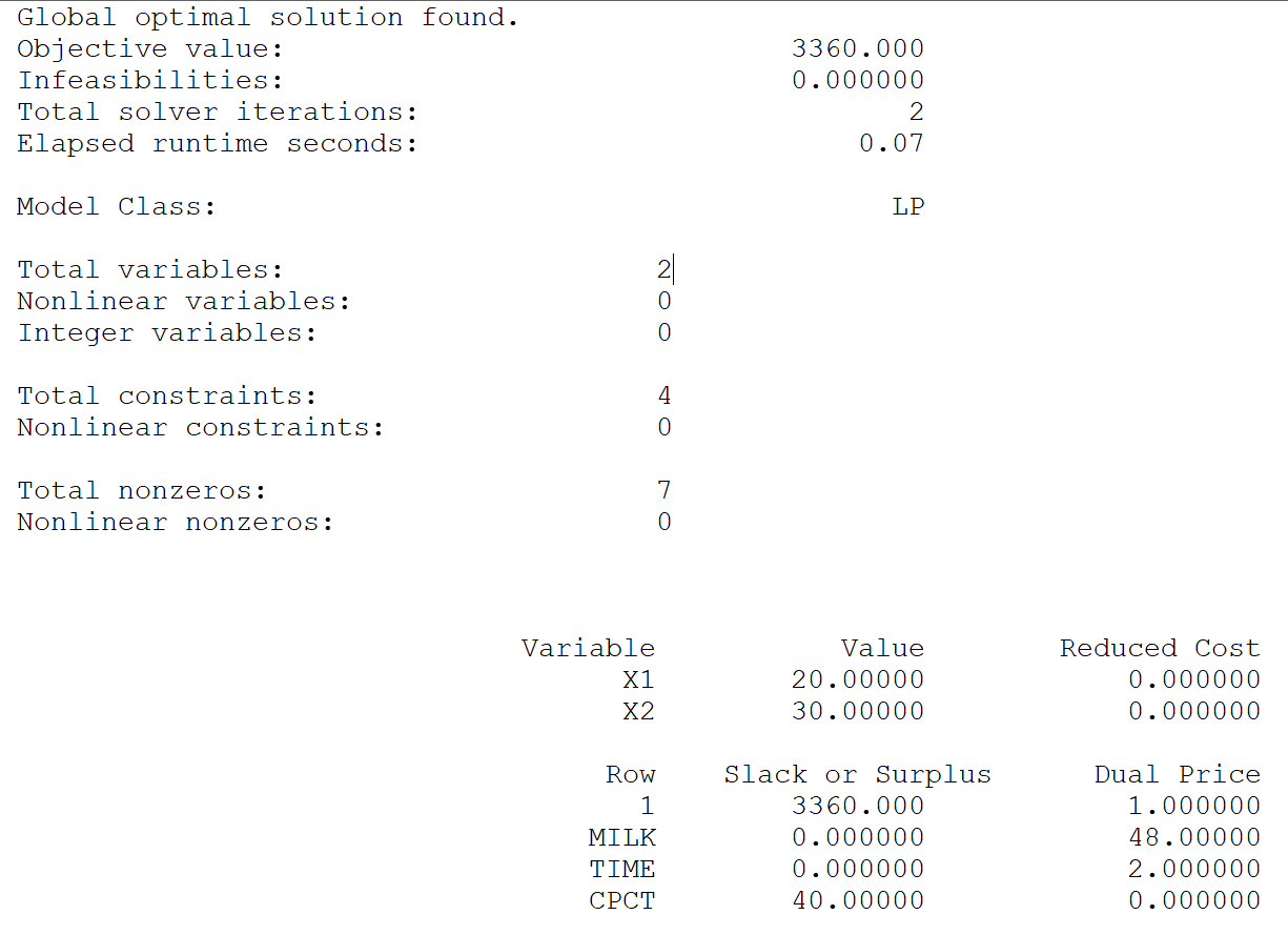
求得最优解为 $(x_1,x_2)=(20,30)$, 此时最优值为 $z=3360$.
Slack or Surplus 指松弛或剩余, 也就是资源的剩余. 这里[MILK]和[TIME]均没有剩余, 只有[CPCT]有富余的量 40, 即甲车间只生产了 $20*3$ 公斤的 $A_1$, 离最大加工量 100kg 还有富余 40kg.
影子价格(Dual Price)
所谓的影子价格, 指当某种资源增加一个单位时, 效益的增加量. 当然, 在其他资源是固定的情况下.
比如, 这里考虑 [MILK] 的影子价格. 记 $x_1+x_2=m$.
\[
z=72x_1+64x_2\\
x_1+x_2=m\\
12x_1+8x_2=480\\
\]
于是, $x_2=60-\frac{3}{2}x_1$, 代入第(2)式, 得
\[
x_1+60-\frac{3}{2}x_1=m,
\]
推出
\[
x_1=120-2m.
\]
于是
\[
\begin{split}
z&=72x_1+64(60-\frac{3}{2}x_1)\\
&=3840-24x_1\\
&=3840-24(120-2m)\\
&=960+48m.
\end{split}
\]
因此, $\frac{dz}{dm}=48$. 也就是说, 当 $m$ 也就是[MILK]的供应量增加1桶时, 效益 $z$ 就增加 48 元.
因此, 对于第一个问题, 使用 35 元的成本购买一桶牛奶, 将带来 48 元的收益, 当然值得投资, 要买. 至于最多买多少, 那么就涉及到影子价格的有意义范围. 这个称为敏感性分析.
图解法
由于此题只涉及两个变量, 因此可以使用手工计算, 特别是借助图形, 可以直观理解最优解及其他一些概念.
约束条件
\[
x_1+x_2\leqslant 50,\\
12x_1+8x_2\leqslant 480,\\
3x_1\leqslant 100,\\
x_i\geqslant 0,\quad i=1,2.
\]
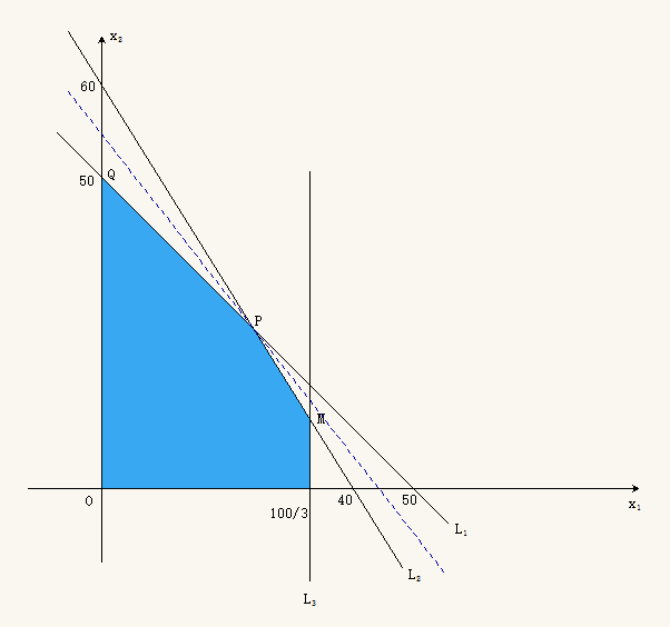
给出了可行域, 如图中的多边形区域.
目标函数 $\max z=72x_1+64x_2$, 若令 $72x_1+64x_2=0$, 则对应的直线是过原点的斜率为 $-\frac{9}{8}$ 的直线. 此斜率介于 $L_1: x_1+x_2=50$ ($k_1=-1$)和 $L_2: 12x_1+8x_2=480$ ($k_2=-\frac{3}{2}$) 之间.
因此, 当将此直线向上平移(或者等价的, 沿 $x_2$ 轴正方向移动), 则 $z$ 的值会越来越大, 当过点 $P$ 时, 直线 $72x_1+64x_2=C$ 为图中蓝色虚线. 此时 $z$ 达到最大值 $C$.
容易求出点 $P$ 的坐标为 $(20,30)$, 此即该问题的最优解. (即求解下面的线性方程组.)
\[
\begin{aligned}
x_1+x_2=50,\\
12x_1+8x_2=480.
\end{aligned}
\]
于是,
\[
\max z=72\cdot 20+64\cdot 30=3360.
\]
目标函数的最优值为 3360元.
End
Thanks very much!